Benchmarking NeST's Refraction Tomography Inversion - Part 1
Comparing our first break refraction tomography inversion to a known near surface model
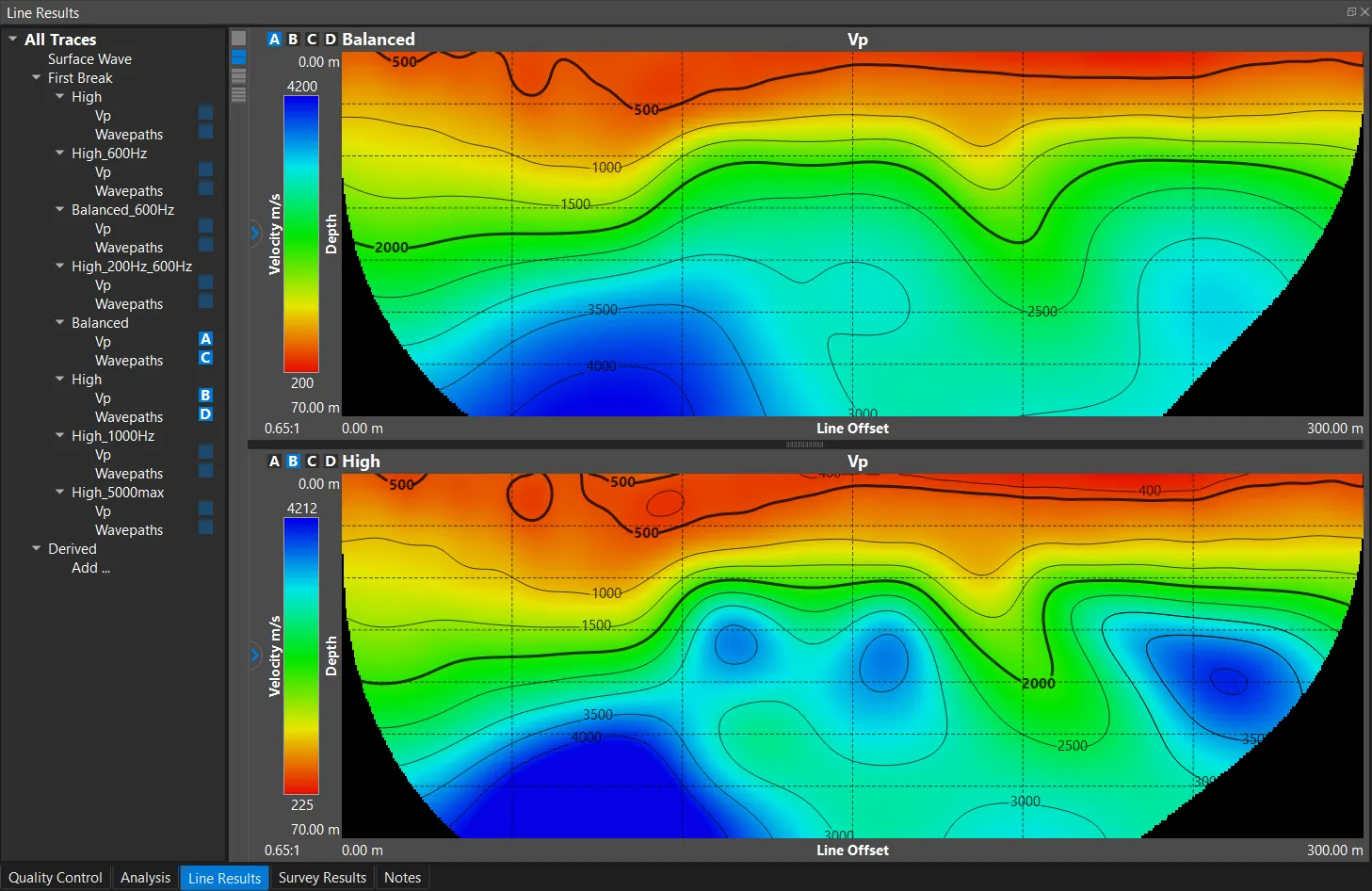
Welcome to our first Benchmark series, where I set out to benchmark our Refraction Tomographic Inversion. Throughout this series, I will systematically test the sensitivity and performance of NeST’s refraction inversion and explore its various parameters using a known near surface velocity model. Additionally, I plan to dive into some of the theory behind our inversion and explain in a little more depth why we made various decisions along the way.
For Part 1, we will keep it simple and lay out some of the background and present our easy “Out of the Box” results.
Basic Inversion Design Breakdown
A deep dive into all of the intricacies and design decisions that went into creating this inversion would likely require I write a textbook. To keep it short, below I have outlined the main summary points that roughly explain our inversion.
Our Refraction Tomographic Inversion is built with:
- Eikonal forward model that includes all possible first arrival wave types (i.e. direct, diving, refracted)
- Wavepath based sensitivity kernels (as opposed to ray based approaches)
- Regularized inversion approach for model update calculations (as opposed to back-projection)
- Wavelength dependent smoother (as opposed to fixed sized moving window based smoothers)
I will expand a bit on these at various points in this series and give some more background on why these different design/implementation decisions were made. I will try to update the above bullets to link to future posts in this series that goes into more depth about them.
The Test Model
We have chosen to use the model specified in Zelt et al. (2013). This model was made available through a general call out to various software providers and research groups, as a type of “Blind Test” to see how well various inversion algorithms and approaches worked to constrain a complex, yet realistic, near surface model. The model is shown below and represents unconsolidated sediments overlying bedrock with variable depth (step in bedrock depth), as well as a steeply dipping fracture zone in the bedrock (representing a fault zone). The other feature to note is the low velocity lens near the surface of the model, which is a notoriously difficult feature to resolve with tomographic inversions.
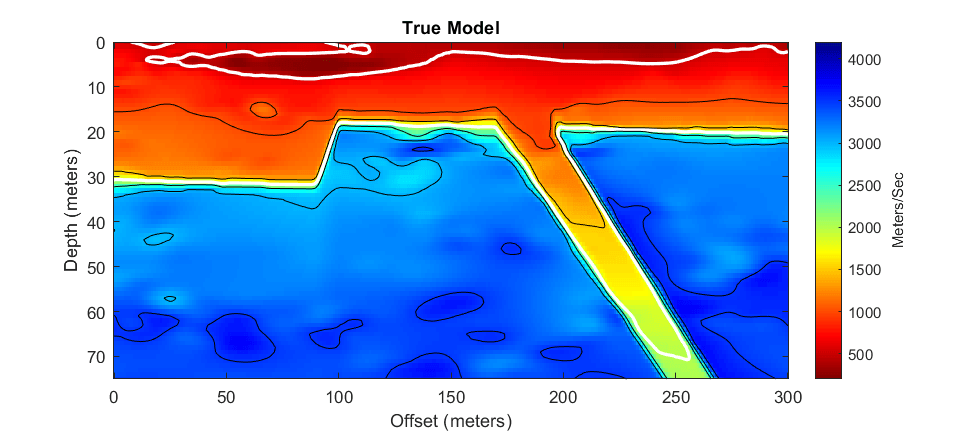 Figure 1: True model from Zelt et al. 2013. White contours are at 500m/s and 2000m/s and are repeated in all velocity model plots to aid in comparison with the true model
The added benefit of using this model, is that our results can be compared to many of the other inversions currently available. Even better, I can extend beyond just qualitative comparisons, but do some quantitative comparisons of our inversion results with other algorithms. Additionally, I have found this model to be used to validate/test other inversion approaches and processing steps in the literature. For those reasons and more, this model will be used for our initial and continued benchmarking.
Existing Results
There are 14 different results that were published in the original publication by Zelt et al. (2013). To avoid any potential copyright infringements, I will not be including any figures from that original publication, but you can potentially view the publication here or can look for other available pdf versions here. I will pull some data out from the publication so I can make some direct comparisons here.
Table 1 below includes the five models who had the lowest (best) measure of misfit in each of the five quantitative comparison metrics. The model numbers in the first column are the same model number found in the original paper. For information on these quantitative metrics, please see the Appendix or the original publication. I will not get into the weeds right now describing what each of these measures may or may not indicate about the final result but I want to highlight one important thing.
Just because a model scores best in one metric, does not automatically indicate that it is a “great” result. For instance, model 8 had the lowest mean difference (average of all the differences between the true and predicted velocity models) but performed very poorly for most other measures (including being one of the worst performers for the mean Relative difference).
To help quantify the quality/performance of each result across all quantitative metrics, I calculated a couple additional rank based metric. I ranked each “Model” in each of the five metrics, and calculated the respective models “Average Rank” (second to last column). I then calculated their “Overall Rank” (last column) by ranking them by the previously calculated “Average Rank” column. This is by no means a perfect measure as it only takes into account their ranks and all metrics are equally weighted; however, this is a better overall measure of how any given model performs (in the future, I will formulate a better general rating scheme).
| Model | T_rms (ms) | Mean diff. (m/s) | Std. dev. (m/s) | Mean rel. diff. (%) | Std. dev. (%) | Best Metric | Average Rank | Overall Rank |
|---|---|---|---|---|---|---|---|---|
| 8 | 1.40 | -16 | 524 | +7.1 | 37.9 | Mean diff. (m/s) | 11.0 | 13 |
| 10 | 1.13 | -111 | 469 | -0.6 | 22.1 | Std. dev. rel. (%) | 3.4 | 1 |
| 11 | 1.05 | -141 | 449 | -1.2 | 24.6 | T_rms (ms) | 4.0 | 2 |
| 12 | 1.20 | -152 | 439 | -1.3 | 22.2 | Std. dev. (m/s) | 4.8 | 3 |
| 14 | 1.59 | -93 | 675 | +0.4 | 27.7 | Mean rel. diff. (%) | 9.2 | 9 |
Table 1: A subset of the models who performed best in one of the 5 quantitative metrics in the original Zelt et al. 2013 paper
NeST Results
For this post, I will only show results from two different inversion runs from NeST. If GeoFennex was around when this blind test happened, these would potentially be the two results that we would have submitted, knowing nothing about the true model.
Default Parameter Inversion
These results come from our default inversion parameters and only adjusting the parameters that were known to us at the beginning including:
- 1 mSec travel time errors
- 100 Hz dominant frequency (I set our Wavelength Dependent Smoother to a frequency of 100 Hz)
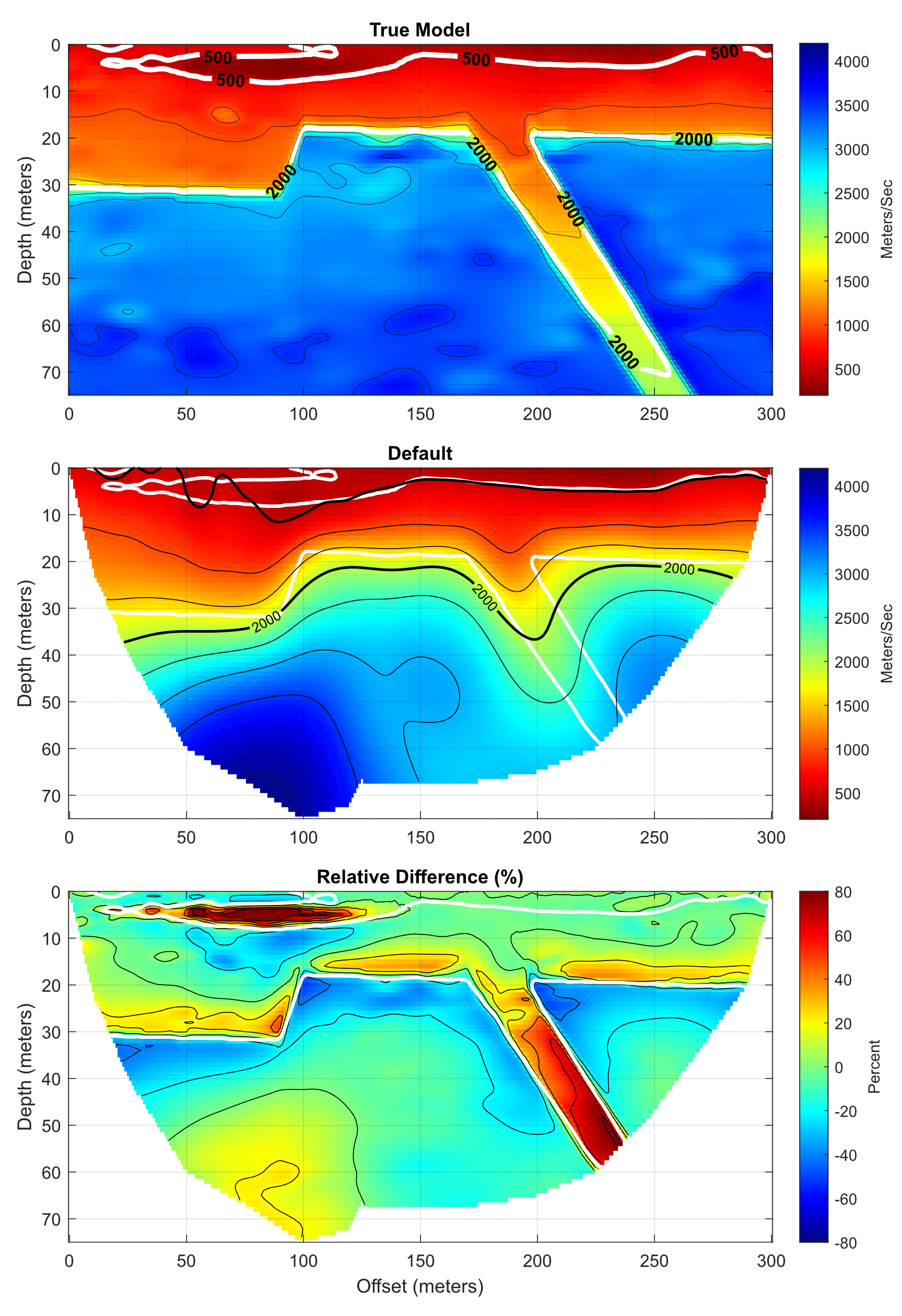 Figure 2: Default inversion parameters. White contours are at 500m/s and 2000m/s from the true model. Middle: Black contours have a 500m/s interval. Bottom: Contour intervals of 20%
From a qualitative perspective, we do a good job resolving all of the features in the model; specifically, the step in the bedrock surface, the presence of the low velocity faulted region, and the correct dip orientation of the faulted region. The only thing that we do not recover well is the shallow velocity inversion/low velocity lens near the surface. I will note for all the original models presented in the original paper, it appears that no result offered a definitive identification of this low velocity lens.
High Resolution Inversion
First a little background to explain this “parameter” change used in this result. While developing and testing our refraction inversion, I explored a variety of ways in which to implement different aspects of the inversion process. I found that much of the literature lacked thorough detail into how different intermediate steps should be implemented. Through the tedious process of figuring out and implementing all of these various steps, I got to the problem of how to handle collecting and applying updates across inversion iterations. I eventually discovered that our updates were largely free of numerical noise, artifacts, and/or instabilities that would normally require the application of an additional smoothing operation. The quality of our model updates meant I had the freedom to try things like collecting unsmoothed updates across all our iterations, offering the potential for a higher resolution final result.
This model run represents the “High” resolution result available from NeST, yielded from nothing more than how we collect and apply updates with no additional smoothing. All other parameters are kept the same.
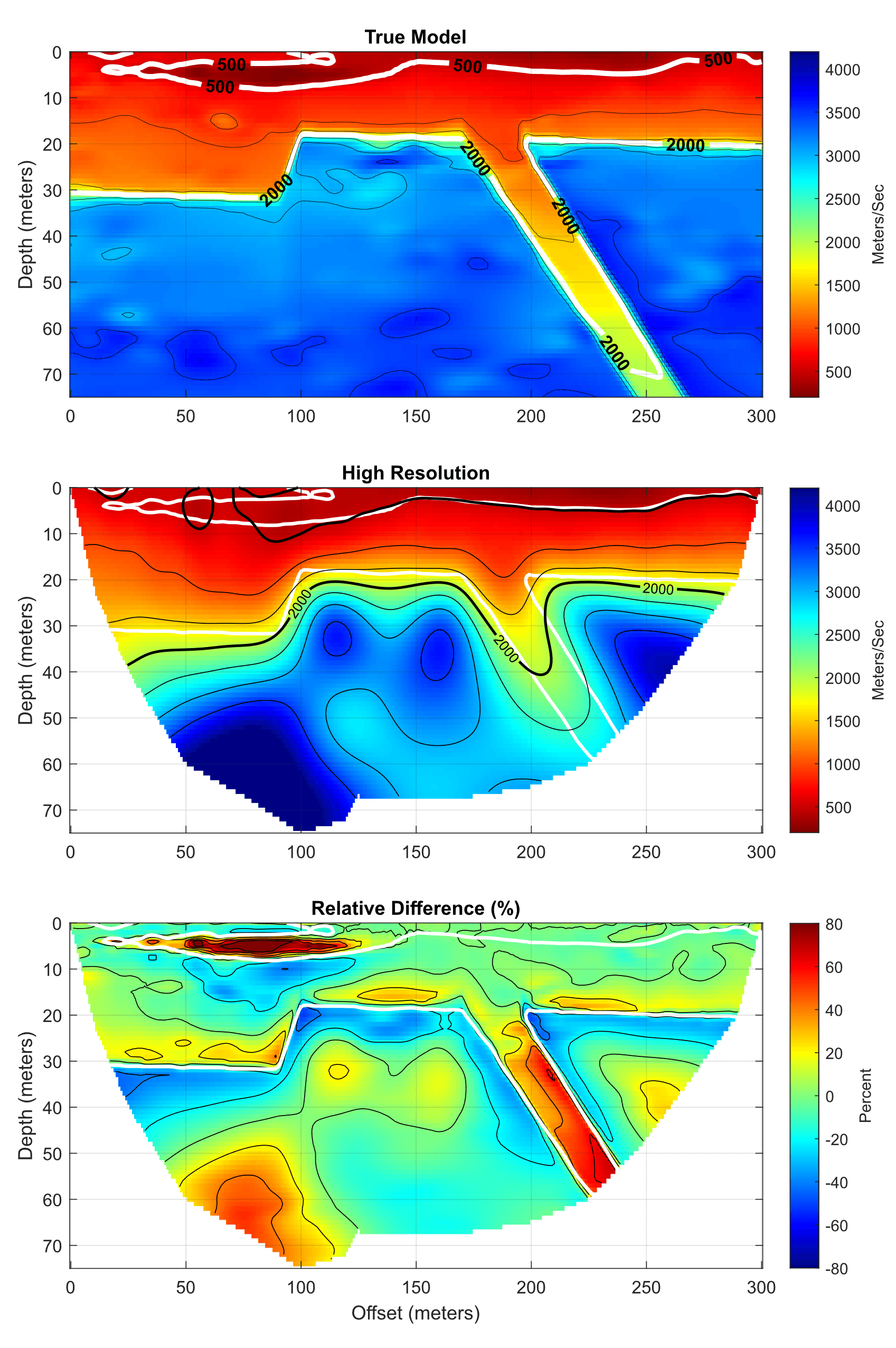 Figure 3: High resolution setting with the rest of the default inversion parameters. White contours are at 500m/s and 2000m/s from the true model. Middle: Black contours have a 500m/s interval. Bottom: Contour intervals of 20%
Like our Default run (figure 2), we correctly resolve the step in the bedrock, and the presence and dip orientation of the faulted region. What the high resolution result also shows, that all previous solutions failed to do, is the definitive identification of the low velocity lens near the surface. Additionally, I would argue that this result offers a higher degree of certainty for an interpreter to correctly identify the bedrock surface and the faulted region due to the greater rate of change in velocities at their respective boundaries (this observation is also supported in the cross-sections presented in figure 4 and figure 5 below).
Fixed Depth and Offset Comparisons
The figures below are another set used in the original Zelt et al. 2013 paper, and act as another means of qualitative comparison via cross-sections. A range of fixed depth and fixed offset cross sections were taken to compare between our results as it is a bit easier to make comparisons between different inversion results.
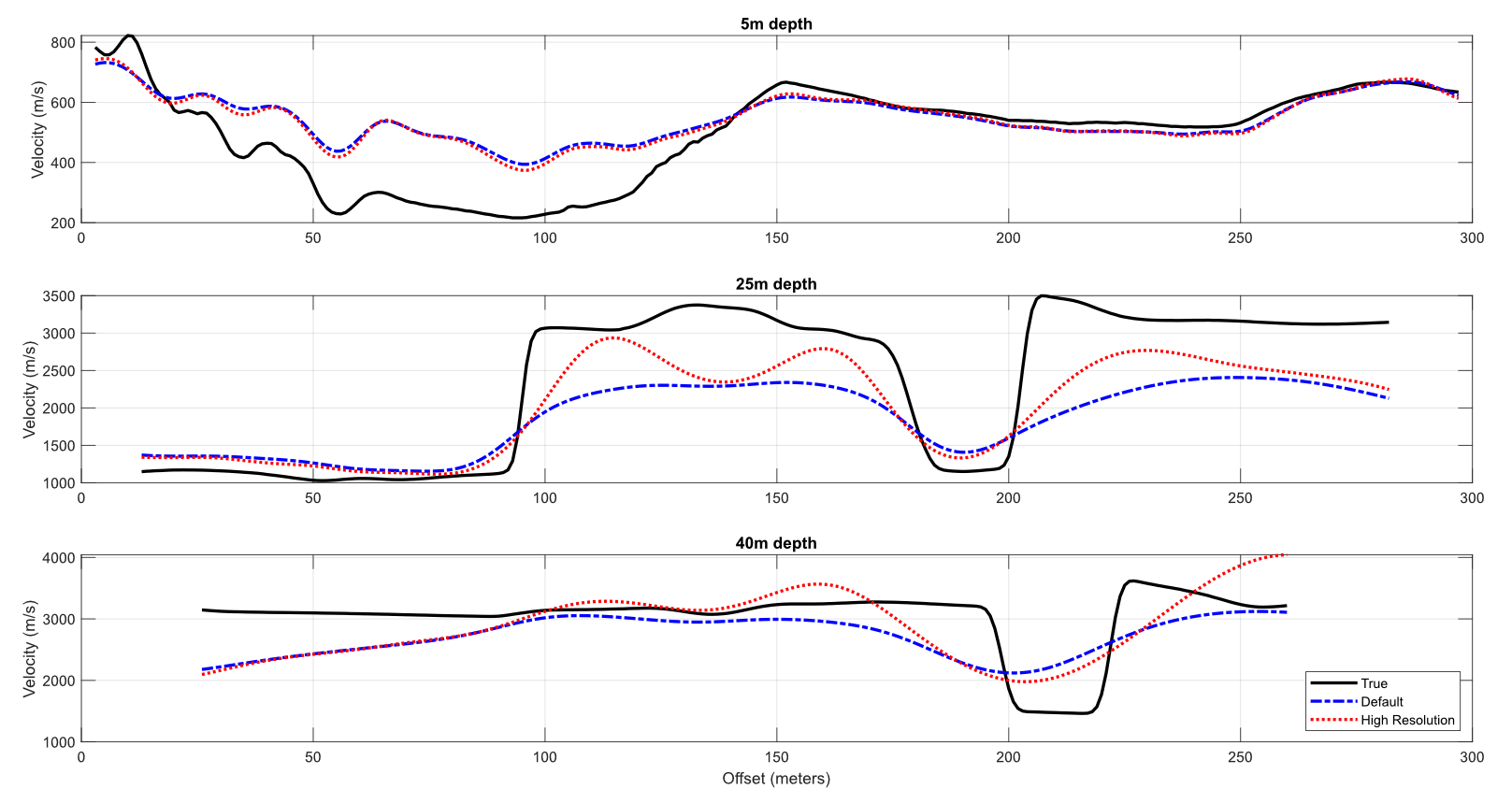 Figure 4: Fixed depth cross section. Black line is the true model. Blue line is our “Default” inversion run and the Red line is our “High resolution” inversion run
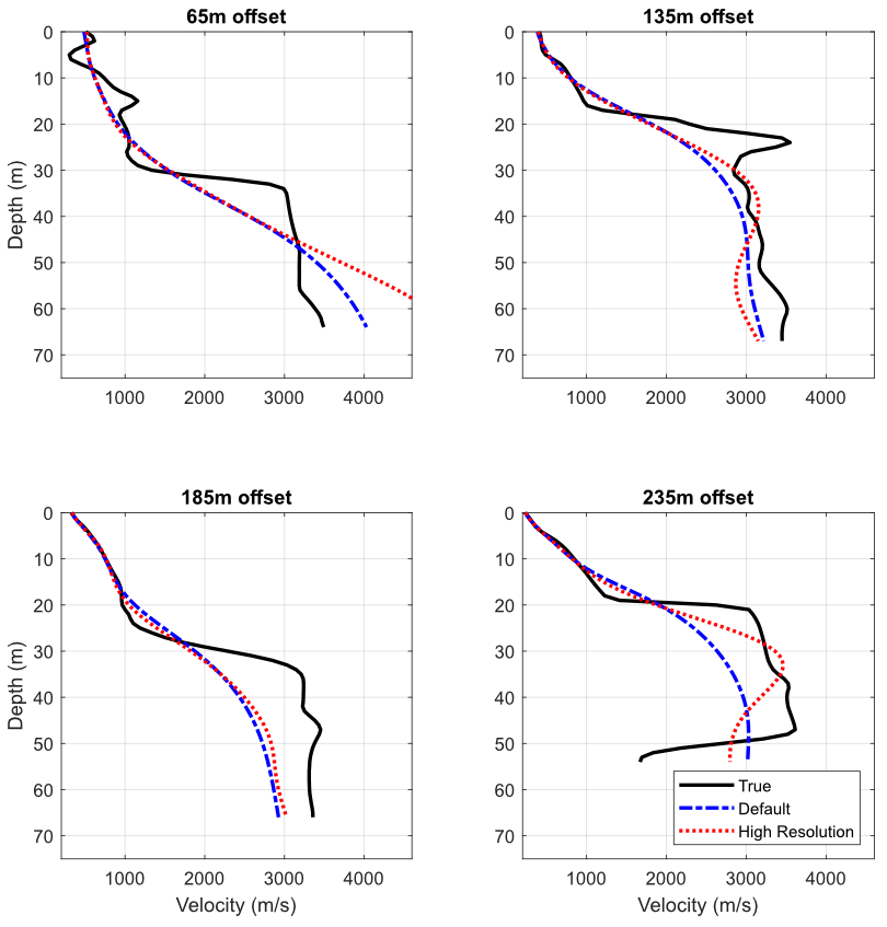 Figure 5: Fixed offset cross section. Black line is the true model. Blue line is our “Default” inversion run and the Red line is our “High resolution” inversion run
These plots will be utilized more in future posts exploring the sensitivities to different inversion parameters, as comparisons will need to be made across a lot more than two inversion results.
Quantitative comparison
The previous qualitative comparisons illustrate the general capabilities of NeST’s refraction tomography inversion to accurately resolve a complex near surface model. To lend some more Quantitative weight to our results, we added our results to Table 1 and recomputed the ranking calculations (see Table 2 below).
Based on the “Average Rank”, our Default inversion result performed as well as the best performing model from the original paper (model 10) and is tied with the High resolution result for the best travel time misfit (T_rms).
The High resolution result outperformed all other results and by a pretty large margin, with an “Average Rank” over one full rank better than the next closest models (Model 10 and NeST’s Default model). The High resolution result additionally scores top rank in travel time misfit (T_rms), mean relative difference (Mean rel. diff. (%)), and the standard deviation of the relative difference (Std. dev. (%)). For information on these quantitative metrics, please see the Appendix.
| Model | T_rms (ms) | Mean diff. (m/s) | Std. dev. (m/s) | Mean rel. diff. (%) | Std. dev. (%) | Best Metric | Average Rank | Overall Rank (incl. NeST) |
|---|---|---|---|---|---|---|---|---|
| 8 | 1.40 | -16 | 524 | +7.1 | 37.9 | Mean diff. (m/s) | 11.8 | 15 |
| 10 | 1.13 | -111 | 469 | -0.6 | 22.1 | - | 4.2 | 2 |
| 11 | 1.05 | -141 | 449 | -1.2 | 24.6 | - | 4.8 | 4 |
| 12 | 1.20 | -152 | 439 | -1.3 | 22.2 | Std. dev. (m/s) | 5.6 | 5 |
| 14 | 1.59 | -93 | 675 | +0.4 | 27.7 | - | 10.2 | 11 |
| Default | 1.01 | -148 | 460 | -2.5 | 21.7 | T_rms | 4.2 | 2 |
| High | 1.01 | -54 | 503 | -0.3 | 21.0 | T_rms, Mean rel. (%), Std. dev. rel. (%) | 2.8 | 1 |
Table 2: Same models shown in Table 1 but updated as if the results presented here were included in the original analysis
Modeling in NeST
You may notice that the images we are showing look suspiciously similar to Matlab figures (and nothing like they came from NeST)… Well you are right in your observations. Our built in Modeling Suite is actively being developed and tested, but will not be available until our next release (2.0). Once the NeST Modeling functionality is completed, everything I am showing could be done within NeST including creating/importing the true models, generating synthetic data (first breaks), running inversions, creating comparison images/graphs between results, and generating figures.
Here is a little taste of how our modeling suite seamlessly integrates into NeST and I am able to use our existing Line Result features to plot and compare across different model runs. This is what I used to generate all of the inversion results presented here and many more that are for future posts in our Benchmark series.
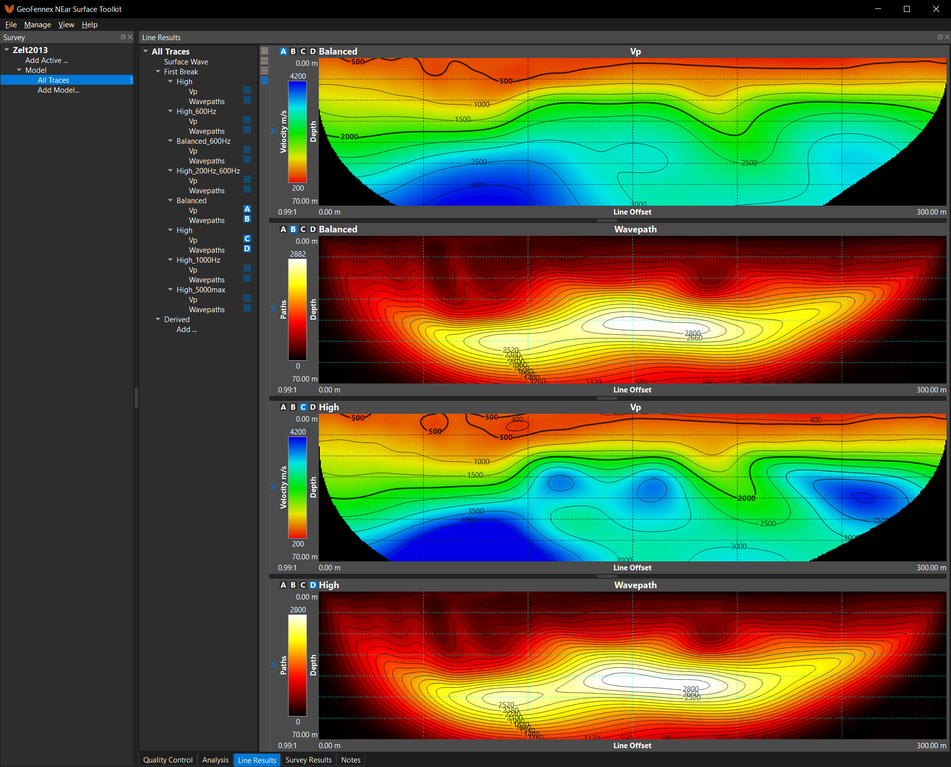 Sneak peak: One of the inversion runs has scored an average rank of 1.2! I will be putting NeST and this inversion through its paces and showing how well it performs.
Citations
- Zelt, Colin A., et al. “Blind test of methods for obtaining 2-D near-surface seismic velocity models from first-arrival traveltimes.” Journal of Environmental and Engineering Geophysics 18.3 (2013): 183-194. doi:10.2113/JEEG18.3.183, PDF Link, Google Scholar Link
Appendix: Quantitative measures
There are five metrics used in the original publication to try to quantify the accuracy of the various approaches and solutions. The shorthand used in the tables above and the longer form description are outlined below:
- T_rms (ms): Root Mean Square traveltime misfit (measure of how well the predicted times match the observed times)
- Mean diff. (m/s): mean of all velocity differences (Predicted Velocity - True Velocity)
- Std. dev. (m/s): standard deviation of velocity differences
- Mean rel. diff. (%): mean of the relative velocity differences ((Predicted Velocity - True Velocity) / True Velocity)
- Std. dev. (%): standard deviation of the relative velocity differences